A gentle introduction to Generalized Linear Models in R

What are generalized linear models?

Generalized linear models (glm) are a special form of linear models used when errors do not follow a normal distribution. In previous posts I’ve discussed linear models (lm), their use and interpretation.

To recap, lm’s model a response variable which depends on one or more independent variables

y~x

  Regular linear models have several assumptions, a really important one is the  normal distribution of errors.  Errors are the differences between the observed and predicted values of the response variable.

Let’s use an example. Let’s say you are modeling the effect of seedling density on seedling herbivory, both measured as continuous variables.

herbivory~density

  If you assume a linear relationship between both variables, a linear model will produce a linear equation that allows us to predict how much herbivory a plant will have based on its local density. Generally such equations are presented in the form:

\[ y \sim \alpha + \beta_1 x \]

With \(\alpha\) as the intercept and \(\beta_1\) as the regression coefficient, which depicts the linear effect of density on herbivory. If \(\beta_1 > 0\) it means that an increase in density will have a positive effect (i.e., increase) herbivory. This relationship is usually displayed as a regression line relating the dependent and independent variables.

  The errors are the differences (dotted lines) between observed values (dots on previous figure) and the regression line. When both variables are normally distributed and linearly related, the distribution of the errors should follow a normal distribution with zero mean.

Comparing two regression slopes by means of an ANCOVA

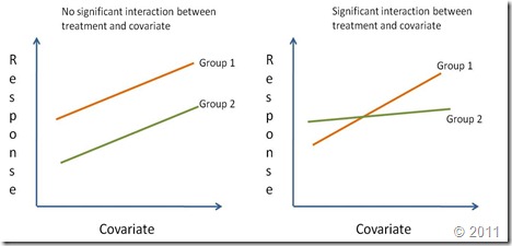
Regressions are commonly used in biology to determine the causal relationship between two variables. This analysis is most commonly used in morphological studies, where the allometric relationship between two morphological variables is of fundamental interest. Comparing scaling parameters (i.e. slopes) between groups can be used by biologist to assess different growth patterns or the development of different forms or shapes between groups. For examples, the regression between head size and body size may be different between males and females if they grow differently. This difference in allometric growth should manifest itself as a different slope in both regression lines.

Ancova

The analysis of covariance (ANCOVA) is used to compare two or more regression lines by testing the effect of a categorical factor on a dependent variable (y-var) while controlling for the effect of a continuous co-variable (x-var). When we want to compare two or more regression lines, the categorical factor splits the relationship between x-var and y-var into several linear equations, one for each level of the categorical factor.
Regression lines are compared by studying the interaction of the categorical variable (i.e. treatment effect) with the continuous independent variable (x-var). If the interaction is significantly different from zero it means that the effect of the continuous covariate on the response depends on the level of the categorical factor. In other words, the regression lines have different slopes (Right graph on the figure below). A significant treatment effect with no significant interaction shows that the covariate has the same effect for all levels of the categorical factor. However, since the treatment effect is important, the regression lines although parallel have different intercepts. Finally, if the treatment effect is not significant nor its interaction with the covariate (but the coariate is significant), this means there is a single regression line. A reaction norm is used to graphically represent the possible outcomes of an ANCOVA.

For this example we want to determine how body size (snout-vent length) relates to pelvic canal width in both male and female alligators (data from Handbook of Biological Statistics). In this specific case, sex is a categorical factor with two levels (i.e. male and female) while snout-vent length is the regressor (x-var) and pelvic canal width is the response variable (y-var). The ANCOVA will be used to assess if the regression between body size and pelvic width are the comparable between the sexes.

Interpretation

An ANCOVA is able to test for differences in slopes and intercepts among regression lines. Both concepts have different biological interpretations. Differences in intercepts are interpreted as differences in magnitude but not in the rate of change. If we are measuring sizes and regression lines have the same slope but cross the y-axis at different values, lines should be parallel. This means that growth is similar for both lines but one group is simply larger than the other. A difference in slopes is interpreted as differences in the rate of change. In allometric studies, this means that there is a significant change in growth rates among groups.
Slopes should be tested first, by testing for the interaction between the covariate and the factor. If slopes are significantly different between groups, then testing for different intercepts is somewhat inconsequential since it is very likely that the intercepts differ too (unless they both go through zero). Additionally, if the interaction is significant testing for natural effects is meaningless (see The Infamous Type III SS). If the interaction between the covariate and the factor is not significantly different from zero, then we can assume the slopes are similar between equations. In this case, we may proceed to test for differences in intercept values among regression lines.

Performing an ANCOVA

For an ANCOVA our data should have a format very similar to that needed for an Analysis of Variance. We need a categorical factor with two or more levels (i.e. sex factor has two levels: male and female) and at least one independent variable and one dependent or response variable (y-var).

> head(gator)
sex snout pelvic
1 male  1.10   7.62
2 male  1.19   8.20
3 male  1.13   8.00
4 male  1.15   9.60
5 male  0.96   6.50
6 male  1.19   8.17

The preceding code shows the first six lines of the gator object which includes three variables: sex, snout and pelvic, which hold the sex, snout-vent size and the pelvic canal width of alligators, respectively. The sex variable is a factor with two levels, while the other two variables are numeric in their type.
We can do an ANCOVA both with the lm() and aov() commands. For this tutorial, we will use the aov() command due to its simplicity.

> mod1 <- aov(pelvic~snout*sex, data=gator)

> summary(mod1)             Df Sum Sq Mean Sq  F value    Pr(>F)
snout        1 51.871  51.871 134.5392 8.278e-13 ***
sex          1  2.016   2.016   5.2284   0.02921 *
snout:sex    1  0.005   0.005   0.0129   0.91013
Residuals   31 11.952   0.386                   
---


Signif. codes:  0 ‘***’ 0.001 ‘**’ 0.01 ‘*’ 0.05 ‘.’ 0.1 ‘ ’ 1 

The previous code shows the ANCOVA model, pelvic is modeled as the dependent variable with sex as the factor and snout as the covariate. The summary of the results show a significant effect of snout and sex, but no significant interaction. These results suggest that the slope of the regression between snout-vent length and pelvic width is similar for both males and females.
A second more parsimonious model should be fit without the interaction to test for a significant differences in the slope.

> mod2 <- aov(pelvic~snout+sex, data=gator)
> summary(mod2)
        Df Sum Sq Mean Sq  F value    Pr(>F)
snout        1 51.871  51.871 138.8212 3.547e-13 ***
sex          1  2.016   2.016   5.3948   0.02671 *
Residuals   32 11.957   0.374                   
---
Signif. codes:  0 ‘***’ 0.001 ‘**’ 0.01 ‘*’ 0.05 ‘.’ 0.1 ‘ ’ 1 

The second model shows that sex has a significant effect on the dependent variable which in this case can be interpreted as a significant difference in ‘intercepts’ between the regression lines of males and females. We can compare mod1 and mod2 with the anova() command to assess if removing the interaction significantly affects the fit of the model:

> anova(mod1,mod2)
Analysis of Variance Table

Model 1: pelvic ~ snout * sex
Model 2: pelvic ~ snout + sex
Res.Df    RSS Df  Sum of Sq      F Pr(>F)
1     31 11.952                        
2     32 11.957 -1 -0.0049928 0.0129 0.9101

The anova() command clearly shows that removing the interaction does not significantly affect the fit of the model (F=0.0129, p=0.91). Therefore, we may conclude that the most parsimonious model is mod2. Biologically we observe that for alligators, body size has a significant and positive effect on pelvic width and the effect is similar for males and females. However, we still don’t know how the slopes change.
At this point we are going to fit linear regressions separately for males and females. In most cases, this should have been performed before the ANCOVA. However, in this example we first tested for differences in the regression lines and once we were certain of the significant effects we proceeded to fit regression lines.
To accomplish this, we are now going to sub-set the data matrix into two sets, one for males and another for females. We can do this with the subset() command or using the extract functions []. We will use both in the following code for didactic purposes:

> machos <- subset(gator, sex=="male")
> hembras <- gator[gator$sex=='female',]

Separate regression lines can also be fitted using the subset option within the lm() command, however we will use separate data frames to simplify the creation of graphs:

> reg1 <- lm(pelvic~snout, data=machos); summary(reg1)
Call:
lm(formula = pelvic ~ snout, data = machos)

Residuals:
 Min       1Q   Median       3Q      Max
-0.85665 -0.40653 -0.08933  0.04518  1.57408

Coefficients:
        Estimate Std. Error t value Pr(>|t|)
(Intercept)   0.4527     0.9697   0.467    0.647
snout         6.5854     0.8625   7.636 6.85e-07 ***
---
Signif. codes:  0 ‘***’ 0.001 ‘**’ 0.01 ‘*’ 0.05 ‘.’ 0.1 ‘ ’ 1

Residual standard error: 0.7085 on 17 degrees of freedom
Multiple R-squared: 0.7742, Adjusted R-squared: 0.761
F-statistic:  58.3 on 1 and 17 DF,  p-value: 6.846e-07

> reg2 <- lm(pelvic~snout, data=hembras); summary(reg2)
Call:
lm(formula = pelvic ~ snout, data = hembras)

Residuals:
 Min       1Q   Median       3Q      Max
-0.69961 -0.19364 -0.07634  0.04907  1.15098

Coefficients:
        Estimate Std. Error t value Pr(>|t|)
(Intercept)  -0.2199     0.9689  -0.227    0.824
snout         6.7471     0.9574   7.047  5.8e-06 ***
---
Signif. codes:  0 ‘***’ 0.001 ‘**’ 0.01 ‘*’ 0.05 ‘.’ 0.1 ‘ ’ 1

Residual standard error: 0.4941 on 14 degrees of freedom
Multiple R-squared: 0.7801, Adjusted R-squared: 0.7644
F-statistic: 49.67 on 1 and 14 DF,  p-value: 5.797e-06 

The regression lines indicate that males have a higher intercept (a=0.45) than females (a=-0.2199), which means that males are larger. We can now plot both regression lines as follows:

> plot(pelvic~snout, data=gator, type='n')
> points(machos$snout,machos$pelvic, pch=20)
> points(hembras$snout,hembras$pelvic, pch=1)
> abline(reg1, lty=1)
> abline(reg2, lty=2)
> legend("bottomright", c("Male","Female"), lty=c(1,2), pch=c(20,1) )

The resulting plot shows the regression lines for males and females on the same plot.

Advanced

We can fit both regression models with a single call to the lm() command using the nested structure of snout nested within sex (i.e. sex/snout) and removing the single intercept for the model so that separate intercepts are fit for each equation.

> reg.todo <- lm(pelvic~sex/snout - 1, data=gator)
> summary(reg.todo)
Call:
lm(formula = pelvic ~ sex/snout - 1, data = gator)
Residuals:
  Min       1Q   Median       3Q      Max
-0.85665 -0.33099 -0.08933  0.05774  1.57408
Coefficients:
             Estimate Std. Error t value Pr(>|t|)
sexfemale        -0.2199     1.2175  -0.181    0.858
sexmale           0.4527     0.8498   0.533    0.598
sexfemale:snout   6.7471     1.2031   5.608 3.76e-06 ***
sexmale:snout     6.5854     0.7558   8.713 7.73e-10 ***
---
Signif. codes:  0 ‘***’ 0.001 ‘**’ 0.01 ‘*’ 0.05 ‘.’ 0.1 ‘ ’ 1
Residual standard error: 0.6209 on 31 degrees of freedom
Multiple R-squared: 0.9936,     Adjusted R-squared: 0.9928
F-statistic:  1213 on 4 and 31 DF,  p-value: < 2.2e-16

Conclusion

The results shown in the previous figure are consistent with our previous findings, pelvic width is positively related to snout-vent length. The relationship is linear for both males and females. The regression slope is positive and similar for both males and females (b ≈ 7.07; weighted average), which means that pelvic width grows faster than snout-vent length. Finally, the regression line of males intercepts with the y-axis at a higher value than for females, which means that males are larger.